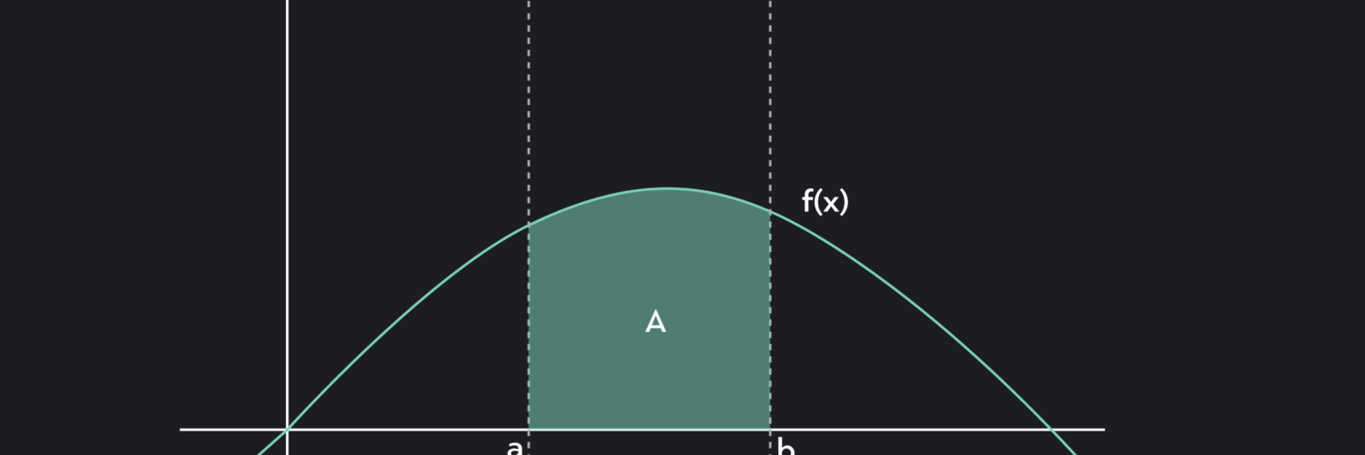
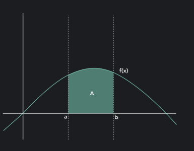
A curved graph can look too smooth to measure with ordinary geometry. Rectangles, on the other hand, are easy: width times height. A Riemann sum connects those two facts by slicing a curved area into many narrow rectangles, adding their areas, and watching the estimate improve as the slices get thinner.
That simple idea sits underneath one of the most important meanings of a definite integral. Before an integral becomes a symbol to evaluate with an antiderivative, it is a careful way to describe accumulation: distance from changing speed, water from changing flow, profit from changing revenue, or area under a curve that does not have straight edges. Riemann sums make that meaning visible.
Why Rectangles Can Estimate a Curve
Suppose a graph shows a function such as $f(x)=x^2$ from $x=0$ to $x=4$. The region under the curve is not a rectangle, triangle, or any basic shape from geometry. Still, the interval from 0 to 4 can be divided into smaller pieces, and each piece can be given a rectangle whose height comes from the function.
The width of each rectangle is the size of a small interval on the x-axis. The height is the value of the function at some chosen point in that interval. Multiplying width by height gives the area of one rectangle. Adding all the rectangle areas gives an estimate for the total area under the curve.
This works because a smooth curve does not change wildly over a very tiny interval. Over a wide interval, one rectangle may miss a lot of the curve. Over a narrow interval, the top of the rectangle follows the curve more closely. The estimate is not magic; it is a controlled approximation.

Left, Right, and Midpoint Sums
A Riemann sum needs a rule for choosing each rectangle’s height. In a left Riemann sum, the height comes from the left endpoint of each subinterval. In a right Riemann sum, the height comes from the right endpoint. In a midpoint sum, the height comes from the middle of each subinterval.
The choice matters most when the function is changing quickly. If a function is increasing, left rectangles usually sit below the curve and underestimate the area, while right rectangles usually reach above much of the curve and overestimate it. If the function is decreasing, the pattern reverses. Midpoint rectangles often balance the error better because each rectangle is centered in its interval.
For example, imagine estimating the area under $f(x)=x^2$ from 0 to 4 using four equal rectangles. Each rectangle has width 1. A left sum uses heights $f(0)$, $f(1)$, $f(2)$, and $f(3)$, so the estimate is $1(0+1+4+9)=14$. A right sum uses $f(1)$, $f(2)$, $f(3)$, and $f(4)$, giving $1(1+4+9+16)=30$.
Those two answers are far apart because four rectangles are still quite rough for a curve that bends upward. Using eight rectangles, then sixteen, then many more, narrows the gap. The important lesson is not that one early estimate is perfect. It is that a repeatable process can get closer and closer to the value the integral represents.
The Formula Behind the Sum
The usual compact form of a Riemann sum looks like this: $\sum_{i=1}^{n} f(x_i^*)\Delta x$. The sigma symbol means to add many terms. The expression $\Delta x$ is the width of each subinterval when the interval is divided evenly. The value $x_i^*$ is the chosen sample point inside the $i$th subinterval.
If the full interval runs from $a$ to $b$ and is divided into $n$ equal parts, then $\Delta x=\frac{b-a}{n}$. Each term $f(x_i^*)\Delta x$ is one rectangle’s area. The sigma notation keeps the repeated addition from becoming a long row of nearly identical terms.
For $f(x)=x^2$ on $[0,4]$, a right Riemann sum with $n$ rectangles uses $\Delta x=\frac{4}{n}$. The right endpoint of the $i$th interval is $x_i=\frac{4i}{n}$. The sum becomes $\sum_{i=1}^{n}\left(\frac{4i}{n}\right)^2\frac{4}{n}$. That may look more complicated than the graph, but it says exactly the same thing: square each chosen x-value, multiply by the small width, and add the rectangles.
Students often first meet sigma notation as if it were a new kind of algebra. It helps to read it more plainly. A Riemann sum is repeated rectangle area. The formula is only a tidy way to track the repetition.
From Estimate to Definite Integral
A definite integral appears when the rectangles become infinitely thin in the limiting sense used in calculus. The notation $\int_a^b f(x)\,dx$ represents the limit of Riemann sums as $n$ grows without bound and the rectangle widths shrink toward zero. The symbol may look very different from the sigma expression, but the idea has not changed: add many tiny contributions over an interval.
This is why the $dx$ at the end of an integral is more than decoration. It points back to the tiny width from the rectangle picture. In a beginner’s first problems, $dx$ also tells which variable is being used. Later, it becomes part of the language of very small changes and accumulation.
The definite integral can give area, but only when the function stays above the x-axis. More generally, it gives signed accumulation. A region above the x-axis contributes positively, while a region below contributes negatively. That distinction matters in velocity problems, where positive and negative values can represent motion in opposite directions.
The Fundamental Theorem of Calculus gives a faster way to compute many definite integrals using antiderivatives. That shortcut is powerful, but it does not replace the rectangle idea. The theorem works because the integral has already been defined as the limit of accumulated tiny changes.
A Worked Example With Changing Speed
Area under a curve can feel abstract until the y-values mean something familiar. Suppose a cyclist’s speed over four seconds is modeled by $v(t)=2t+1$, where speed is measured in meters per second and time is measured in seconds. The area under the speed graph estimates distance traveled.
Use four right rectangles on the interval $[0,4]$. Each rectangle has width $\Delta t=1$. The right endpoints are $t=1,2,3,4$. The speeds are $v(1)=3$, $v(2)=5$, $v(3)=7$, and $v(4)=9$. The Riemann sum is $1(3+5+7+9)=24$, so the right-endpoint estimate is 24 meters.
Because the speed function is increasing, this right sum overestimates the distance over each one-second interval. A left sum would use $t=0,1,2,3$, giving speeds $1,3,5,7$ and an estimate of 16 meters. The true distance lies between those estimates. With more, narrower rectangles, the left and right estimates move closer together.
The exact integral is $\int_0^4(2t+1)\,dt=20$, so the true distance is 20 meters. The rectangle estimates were not wasted work. They show what the integral is measuring before the antiderivative calculation gives the exact value.
Common Mistakes to Watch For
The most common mistake is mixing up width and height. The width comes from the x-interval, such as $\Delta x$ or $\Delta t$. The height comes from the function value, such as $f(x_i)$ or $v(t_i)$. Multiplying two heights or adding function values without the width changes the meaning of the calculation.
Another mistake is forgetting which endpoint rule is being used. Left and right sums can give noticeably different estimates, especially with only a few rectangles. A careful table with columns for interval, chosen x-value, function value, and rectangle area can prevent many errors.
Units also reveal whether the calculation makes sense. If a graph shows velocity in meters per second and time in seconds, each rectangle has units $(\text{meters per second})(\text{seconds})$, which simplifies to meters. The integral then represents distance or displacement, not speed. This is one reason Riemann sums are useful beyond pure math: they keep the units of accumulation honest.
Riemann sums are not just a temporary classroom trick before the real calculus begins. They explain why definite integrals work, why area can represent total change, and why adding many small pieces can measure something smooth. Once that picture is clear, the integral sign feels less like a mysterious symbol and more like a compact record of a careful idea.


Add comment