
 Akshay Dinesh
A calculus optimization problem begins with a simple question: what is the best possible value under these conditions? The word best might mean the largest area, the smallest cost, the shortest time, the greatest profit, or the least amount of material. What makes the problem feel tricky is that the best value is usually not stated directly. It has to be built from the information in the situation.
Derivatives make these problems powerful because they describe how a quantity is changing. If a function is still increasing, its value is not yet as large as it can be. If it is still decreasing, it has not reached its smallest possible value. The most interesting points often happen where the increase slows to zero, where the function changes direction, or where an endpoint limits what is allowed.
That is why optimization is not just a formula hunt. It is a modeling task. The hard part is often turning a story into one function of one variable, with a clear domain, before taking any derivative at all.
Why Optimization Problems Need a Model First
In an ordinary derivative exercise, the function is usually given. You might be asked to differentiate \(f(x)=x^3-6x^2+9x\), find where \(f'(x)=0\), and describe what happens there. An optimization problem hides the function inside a real situation, so the first job is to decide what quantity is being optimized and what information connects the variables.
Suppose a farmer has 100 meters of fencing and wants to make a rectangular pen against a long straight wall. The wall forms one side, so the fence only covers the two widths and the far length. If the width is \(x\), then the length is \(100-2x\). The area is not just “length times width” in the abstract. It becomes a one-variable function: \(A(x)=x(100-2x)\).
That step is the heart of the problem. The rectangle could have many different shapes, but the amount of fencing creates a constraint. Once the constraint turns the area into one function, calculus can ask where that function reaches its greatest value.
Good setup also protects against impossible answers. In the fencing example, \(x\) cannot be negative, and \(100-2x\) must be positive, so the useful domain is \(0<x<50\). A number outside that interval might come from algebra, but it would not describe a real pen.
How Derivatives Locate Possible Best Values
After the model is built, the derivative shows where the output stops increasing or decreasing. For the fencing example, \(A(x)=100x-2x^2\), so \(A'(x)=100-4x\). Setting the derivative equal to zero gives \(100-4x=0\), so \(x=25\). The length is then \(100-2(25)=50\), giving an area of \(1250\) square meters.
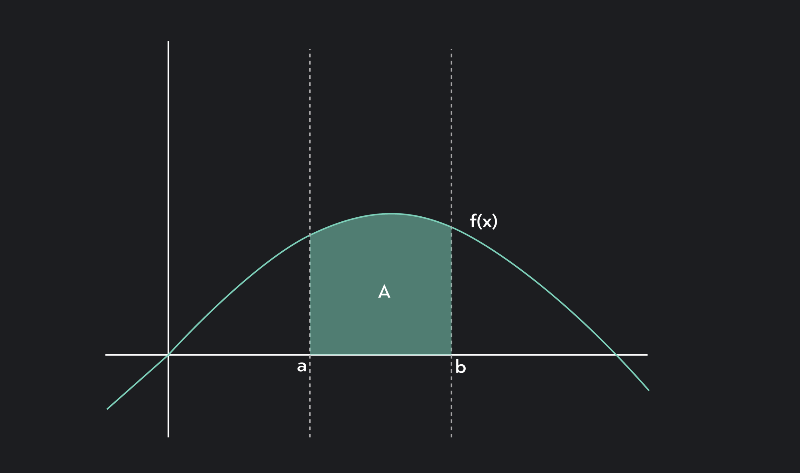
The reason this works is visual as well as algebraic. The graph of \(A(x)\) is a downward-opening parabola. It climbs, flattens at the top, and then falls. At the top, the tangent slope is zero, which is exactly what the derivative detects.
A derivative equal to zero does not automatically mean the problem is solved, though. It only identifies a candidate. Some critical points are maximums, some are minimums, and some are neither. A flat spot on a road might be the crest of a hill, the bottom of a valley, or just a level stretch before the road keeps going.
That is why optimization problems usually need a check after the derivative work. The second derivative can show concavity. A sign chart can show whether the function changes from increasing to decreasing. Endpoint values may also matter, especially when the domain is closed, such as \(0\leq x\leq 50\).
The Constraint Is Usually the Key
Many students get stuck because they start differentiating before they have used the constraint. In most optimization problems, the goal formula begins with more than one variable. Area might be \(A=lw\). Volume might be \(V=lwh\). Cost might depend on distance, material, or speed. The constraint is what reduces that formula to one variable.
Consider an open-top box made by cutting equal squares from the corners of a rectangular sheet and folding up the sides. The volume depends on the cut size and the remaining length and width. If the sheet measures 20 by 30 centimeters and each corner square has side length \(x\), the box has height \(x\), length \(30-2x\), and width \(20-2x\). The volume function is \(V(x)=x(30-2x)(20-2x)\).
This is a classic example because the physical action creates the algebra. Cutting larger squares makes the box taller, but it also shrinks the base. A tiny cut gives a shallow box. A huge cut leaves almost no base. Somewhere between those extremes is a volume that is largest.
The same idea appears outside classroom geometry. A company might balance price and demand, an engineer might reduce material while keeping strength, and a commuter might compare route length against traffic speed. The derivative is useful only after the situation has been translated into a function that honestly represents the tradeoff.
Endpoints Can Beat Critical Points
One common mistake is assuming the answer must come from \(f'(x)=0\). That is often true in a simple textbook example, but a best value can also occur at the edge of what the problem allows. If a function is increasing across the entire allowed interval, its maximum happens at the right endpoint. If it is decreasing the whole way, its minimum happens at the right endpoint instead.
Imagine a store can sell between 100 and 500 tickets because of room capacity and minimum staffing needs. A profit function might have a critical point at 620 tickets, but that number is not allowed. If profit keeps rising throughout the real interval, the best permitted choice is 500 tickets, not 620. The real-world restriction matters as much as the algebra.

Endpoints are especially important when the domain is a closed interval. The safest method is to list all candidates: critical points inside the interval and endpoints on the boundary. Then evaluate the original function at each candidate. The largest output is the absolute maximum, and the smallest output is the absolute minimum.
This approach may feel slower, but it prevents a very common error. A derivative tells where change behaves in a special way. It does not, by itself, know which values the original problem permits.
A Reliable Way to Solve Optimization Problems
A strong optimization solution usually follows a steady pattern. First, name the quantity you want to optimize. Then write a formula for that quantity. If the formula has more than one variable, use the constraint to rewrite it with one variable. After that, identify the domain, take the derivative, find critical points, and compare the candidates.
For the fencing problem, the target quantity was area. The constraint was the available fencing. The one-variable function was \(A(x)=x(100-2x)\), and the domain came from the fact that both dimensions had to be positive. The derivative located \(x=25\), and the shape of the graph confirmed that it produced a maximum rather than a minimum.
For a box-volume problem, the same pattern works even though the algebra is messier. The target quantity is volume. The constraint is the sheet size and the equal corner cuts. The domain comes from the requirement that all dimensions remain positive. The derivative then searches within that domain, not in an unlimited algebraic universe.
- Target: decide what should be largest or smallest.
- Constraint: use the condition that links the variables.
- Function: rewrite the target as one expression in one variable.
- Domain: keep only values that make sense in the situation.
- Derivative: find critical points and compare them with endpoints.
What Optimization Teaches About Calculus
Optimization problems show why derivatives are more than a symbolic skill. A derivative can describe the moment when a useful quantity changes direction, when growth stops being worth the cost, or when a design reaches its best balance. The answer is not only a number; it is a decision supported by a model.
They also show why assumptions matter. A model may ignore friction, waste, changing demand, construction limits, or other details in order to focus on one main relationship. That does not make the model useless. It simply means the answer belongs to the conditions that were chosen.
When optimization feels confusing, the best move is usually to slow down before the derivative. Draw the situation, label the variables, write the constraint in plain algebra, and check the domain. Once the model is clear, the calculus often becomes the easier part. The derivative can find the turning point, but the setup tells it what problem it is actually solving.